Accelerated first-order methods as span-based first-order methods: conversion between momentum form and standard form
Shuvomoy Das Gupta
July 23, 2023
In this blog, we discuss how to write accelerated first-order methods as span-based first-order methods.
Table of contents
Converting between momentum-form and and standard form of span-based first-order method
Consider a \(L\)-smooth function. Span-based first order methods for this function \(f\) are algorithms of the form (called the standard form)
\[x_{k}=x_{0}-\sum_{j=0}^{k-1}\frac{h_{k,j}}{L}\nabla f(x_{j}),\quad\textrm{(SBFOM)}\] where \(k\in\{1,\ldots,N\}\) and \(x_0\) is the initial point.
Also, we have the following "momentum form" of the span-based first-order method, where \(i\in \{0,\ldots, N-1\}\).
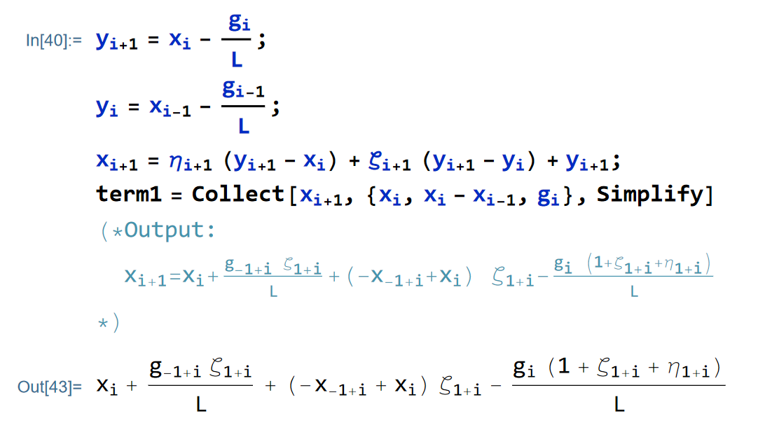
\[ \begin{align*} \begin{array}{ll} y_{i+1} & =x_{i}-\frac{1}{L}\nabla f(x_{i})\\ x_{i+1} & =y_{i+1}+\zeta_{i+1}(y_{i+1}-y_{i})+\eta_{i+1}(y_{i+1}-x_{i}), \end{array}\quad(\textrm{MomentumForm)} \end{align*} \]which we show to be equivalent to (SBFOM). To show that (MomentumForm) is in the form (SBFOM), we put, the iterative form \(y_{+1}\) and \(y_{i}\) in terms of the \(x\) iterates in the second iterate. For simplification purpose, denote \(g_{i}=\nabla f(x_{i})\). We get:
\[ \begin{align*} x_{i+1}=x_{i}+\zeta_{i+1}\left(x_{i}-x_{i-1}\right)-\frac{\left(\zeta_{i+1}+\eta_{i+1}+1\right)}{L}g_{i}+\frac{\zeta_{i+1}}{L}g_{i-1},\quad \textrm{(MOM-SIMP)} \end{align*} \]where the Mathematica code for this is shown below.
Subscript[y, i + 1] = Subscript[x, i] -  Subscript[g, i]/L;
Subscript[y, i] = Subscript[x, i - 1] - Subscript[g, i - 1]/L;
Subscript[x, i + 1] =
  Subscript[\[Eta], i + 1] (Subscript[y, i + 1] - Subscript[x, i]) +
   Subscript[\[Zeta], i + 1] (Subscript[y, i + 1] - Subscript[y, i]) +
    Subscript[y, i + 1];
term1 = Collect[Subscript[x,
 i + 1], {Subscript[x, i], Subscript[x, i] - Subscript[x, i - 1],
  Subscript[g, i]}, Simplify]

(*Output:
    Subscript[x, i] + (
 Subscript[g, -1 + i] Subscript[\[Zeta],
  1 + i])/L + (-Subscript[x, -1 + i] + Subscript[x,
    i]) Subscript[\[Zeta], 1 + i] - (
 Subscript[g,
  i] (1 + Subscript[\[Zeta], 1 + i] + Subscript[\[Eta], 1 + i]))/L
 *)
Now from (SBFOM):
\[\begin{align*} x_{i} & =x_{0}-\sum_{j=0}^{i-1}\frac{h_{i,j}}{L}g_{j},\\ x_{i-1} & =x_{0}-\sum_{j=0}^{i-2}\frac{h_{i-1,j}}{L}g_{j},\end{align*}\] which gives
\[ \begin{align*} x_{i}-x_{i-1} & =-\sum_{j=0}^{i-2}\frac{(-h_{i-1,j}+h_{i,j})}{L}g_{j}-\frac{h_{i,i-1}}{L}g_{i-1}\quad \textrm{(Diff-x)} \end{align*} \]and putting this in (MOM-SIMP) and then simplifying we get:
\[ \begin{align*} & x_{i+1}\\ = & x_{i}-\zeta_{i+1}\sum_{j=0}^{i-2}\frac{\left(h_{i,j}-h_{i-1,j}\right)}{L}g_{j}-\frac{\zeta_{i+1}\left(h_{i,i-1}-1\right)}{L}g_{i-1}-\frac{\left(\zeta_{i+1}+\eta_{i+1}+1\right)}{L}g_{i}, \end{align*} \quad \textrm{(SBFOM-A)} \]where the Mathematica code for the simplification is shown below:
termDif = -\!\(
\*UnderoverscriptBox[\(\[Sum]\), \(j = 0\), \(i - 2\)]
\*FractionBox[\(
\*SubscriptBox[\(g\), \(j\)]\ \((
\*SubscriptBox[\(h\), \(i, j\)] -
\*SubscriptBox[\(h\), \(i - 1, j\)])\)\), \(L\)]\) - (
   Subscript[g, i - 1] Subscript[h, i, i - 1])/L;
term2 = term1 /. ((-Subscript[x, -1 + i] + Subscript[x, i])) ->
    termDif;
term3 = Collect[term2, {Subscript[g, i], Subscript[g, i - 1]},
  Simplify]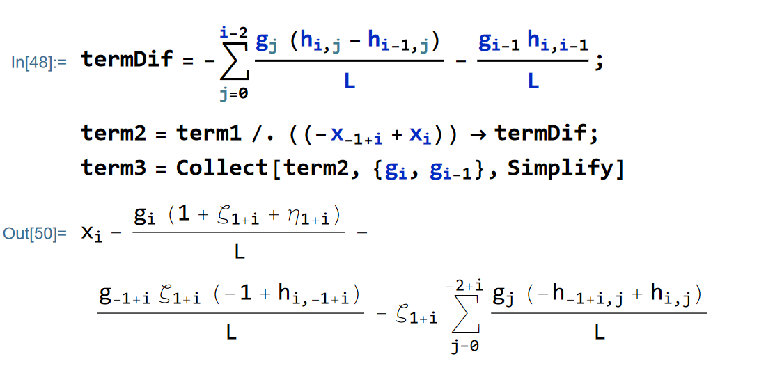
Recall that, using (Diff-x) any (SBFOM) satisfying sequence will obey:
Note that (Diff-x-2) and (SBFOM-A) are in the same format now for a pattern matching. Comparing the terms part by part, we get the following recursive system for \(i\in [0:N-1]\)
\[ \begin{align*}\forall_{j\in[0:i-2]}\quad h_{i+1,j} & -h_{i,j}=\zeta_{i+1}\left(h_{i,j}-h_{i-1,j}\right)\\ h_{i+1,i-1}-h_{i,i-1} & =\zeta_{i+1}\left(h_{i,i-1}-1\right)\\ h_{i+1,i} & =\zeta_{i+1}+\eta_{i+1}+1. \end{align*} \]with initial condition \(h_{1,k}=0\) if \(k<0\) and \(h_{0,k}=0\) for all \(k\). This system of equation gives us a way to compute \(\zeta,\eta\) from \(h\).
Julia code to construct \(h\) from \(\{\zeta, \eta\}\) and back
The main system of equations is for this conversion process is:
\[ \begin{align*} & h\equiv\{h_{i,j}\}_{i\in[1:N],j\in[0:i-1]}\\ & \forall_{i\in[0:N-1]}\forall_{j\in[0:i-2]}\quad h_{i+1,j}-h_{i,j}=\zeta_{i+1}\left(h_{i,j}-h_{i-1,j}\right)\\ & \forall_{i\in[0:N-1]}\quad h_{i+1,i-1}-h_{i,i-1}=\zeta_{i+1}\left(h_{i,i-1}-1\right)\\ & \forall_{i\in[0:N-1]}\quad h_{i+1,i}=\zeta_{i+1}+\eta_{i+1}+1\\ & h_{1,j}=0,\textrm{ if }j<0\\ & \forall_{j\in[0:i-1]}\quad h_{0,j}=0. \end{align*} \]Code to construct \(h\) from \(\{\zeta, \eta\}\)
Suppose we have \(\{\zeta, \eta\}\) and we want to construct \(h\) from that. So, the Julia code to do that is as follows:
## function to construct h from ζ, η

function construct_h_from_ζ_η(N, L, ζ, η; solution_method = :constraint)

   # other option for solution_method is :penalty

   # time to construct model

   mod1 = Model(Gurobi.Optimizer)

   @variable(mod1, h[i=0:N, j=-2:N] >= 0)

   # we are just interested in h[i = 1:N, j = 0:i-1], rest should be set to zero

   for i in 0:N
      for j in -2:N
         if !(i >= 1 && i <= N && j >= 0 && j <= i-1)
            fix(h[i,j], 0.0; force = true)
         end
      end
   end

   if solution_method == :constraint

      for i in 0:N-1
         for j in 0:i-2
            @constraint(mod1, h[i+1,j] - h[i,j] .== ζ[i+1]*(h[i,j] - h[i-1,j]) )
         end
      end

      for i in 0:N-1
         @constraint(mod1, h[i+1,i-1] - h[i,i-1] .== ζ[i+1]*(h[i,i-1] -1) )
      end

      for i in 0:N-1
         @constraint(mod1, h[i+1,i] .== ζ[i+1] + η[i+1] + 1 )
      end

      @objective(mod1, Min, 0)

   elseif solution_method == :penalty

      term_1 = @expression(mod1, sum( (h[i+1,j] - h[i,j] - ζ[i+1]*(h[i,j] - h[i-1,j]))^2 for i in 0:N-1, j in 0:N-1 if j <= i-2) )

      term_2 = @expression(mod1, sum( (h[i+1,i-1] - h[i,i-1] - ζ[i+1]*(h[i,i-1] -1))^2 for i in 0:N-1))

      term_3 = @expression(mod1, sum( (h[i+1,i] - (ζ[i+1] + η[i+1] + 1) )^2 for i in 0:N-1) )

      @objective(mod1, Min, term_1 + term_2 + term_3)

   end

   optimize!(mod1)

   if termination_status(mod1) != OPTIMAL
      @error "termination status is not optimal"
   end

   obj_val = objective_value(mod1)

   @info "Value of h for N=$(N) with fitting error = $(obj_val)"

   h_star = value.(h)

   # h_star_compact = h[i=1:N, j = 0:N-1 if j <= i-1]
   #
   # @show h_star_compact

   return h_star

end
Let us test the function. First, we generate a specific \(\zeta, \eta\) to test for, which comes from OGM (see below about more details about OGM).
## Load the packages

using OffsetArrays, Gurobi, JuMP, LinearAlgebra

N = 5

# Generate θ for OGM

L = 1

R = 1

θ = Dict{Int64,Float64}()

θ[0] = 1

for i in 1:N
   if i <= N-1
        θ[i] = (1+sqrt(1+4*θ[i-1]^2))/2
   elseif i == N
       θ[i] = (1+sqrt(1+8*θ[i-1]^2))/2
   end
end

ζ_OGM = OffsetVector(zeros(N), 1:N)

for i in 0:N-1
   ζ_OGM[i+1] = (θ[i]-1)/θ[i+1]
end

@show ζ_OGM

# output:
# ζ_OGM = [0.0, 0.28175352512532087, 0.434042782780302, 0.5310638054044795, 0.4424791858537259]

η_OGM = OffsetVector(zeros(N), 1:N)

for i in 0:N-1
   η_OGM[i+1] = θ[i]/θ[i+1]
end

@show η_OGM

# output:
# η_OGM = [0.6180339887498948, 0.7376403052281875, 0.7977067398993897, 0.8345650247944008, 0.6352906827290474]
Now let us test the function construct_h_from_ζ_η.
h_star_constraint = construct_h_from_ζ_η(N, L, ζ_OGM, η_OGM; solution_method = :constraint)

@show round.(h_star_constraint[1:N, 0:N-1], digits = 5)

# The output is:
# h_star_constraint[1:N, 0:N-1] =
# [
# 1.61803  0.0      0.0      0.0      0.0;
# 1.79217  2.01939  0.0      0.0      0.0;
# 1.86775  2.46185  2.23175  0.0      0.0;
# 1.90789  2.69683  2.88589  2.36563  0.0;
# 1.92565  2.8008   3.17533  2.96989  2.07777
# ]

h_star_penalty = construct_h_from_ζ_η(N, L, ζ_OGM, η_OGM; solution_method = :penalty)

@show round.(h_star_penalty[1:N, 0:N-1], digits = 5)

# The output is:
# h_star_penalty[1:N, 0:N-1] =
# [
# 1.61803  0.0      0.0      0.0      0.0
# 1.79217  2.01939  0.0      0.0      0.0
# 1.86775  2.46185  2.23175  0.0      0.0
# 1.90789  2.69683  2.88589  2.36563  0.0
# 1.92565  2.8008   3.17533  2.96989  2.07777
# ]

h_star = h_star_penalty # we will use this for another test below
Code to construct \(\{\zeta, \eta\}\) from \(h\)
Now we consider the opposite direction. Now we want to construct \(\{\zeta, \eta\}\) from a given \(h\). The Julia code to do that is as follows:
function construct_ζ_η_from_h(N, L, h; fix_ζ_η = :true, ζ_ws = ζ_OGM, η_ws = η_OGM)

   mod1 = Model(Gurobi.Optimizer)

   @variable(mod1, ζ[i = 1:N])

   @variable(mod1, η[i = 1:N])

   if fix_ζ_η == :true
     @info "fixing  ζ and η to that of OGM to check if there are multiple solutions"
     fix.(ζ, ζ_ws; force=true)
     fix.(η, η_ws; force = true)
  end

   term_1 = @expression(mod1, sum( (h[i+1,j] - h[i,j] - ζ[i+1]*(h[i,j] - h[i-1,j]))^2 for i in 0:N-1, j in 0:N-1 if j <= i-2) )

   term_2 = @expression(mod1, sum( ( h[i+1,i-1] - h[i,i-1] - ζ[i+1]*(h[i,i-1] -1) )^2 for i in 0:N-1))

   term_3 = @expression(mod1, sum( (h[i+1,i] - (ζ[i+1] + η[i+1] + 1) )^2 for i in 0:N-1) )

   @objective(mod1, Min, term_1 + term_2 + term_3)

   optimize!(mod1)

   if termination_status(mod1) != OPTIMAL
      @error "termination status is not optimal"
   end

   obj_val = objective_value(mod1)

   @info "fitting error for N=$(N) to construct ζ, η from h = $(obj_val)"

   ζ_star = value.(ζ)

   η_star = value.(η)

   return ζ_star, η_star

end
Let us now test this function.
ζ_star, η_star = construct_ζ_η_from_h(N, L, h_star; fix_ζ_η = :false)

# output: [ Info: fitting error for N=5 to construct ζ, η from h = -6.039613253960852e-14

@show ζ_star

# output: ζ_star = [6.352740751660148e-16, 0.2817535522830343, 0.43404278553274767, 0.5310638059557159, 0.442479185968013]

@show η_star

# output: η_star = [0.6180340040827577, 0.7376402784557785, 0.7977067372415494, 0.8345650242736313, 0.6352906826136708]
Let us compare now if the original \(\zeta, \eta\) from OGM matches this reconstructed.
## Compare with original ζ, η coming from OGM

@show "difference between ζ_OGM and ζ_reconstructed is: $(norm(ζ_star - ζ_OGM))"

# output:
# "difference between ζ_OGM and ζ_reconstructed is: $(norm(ζ_star - ζ_OGM))" = "difference between ζ_OGM and ζ_reconstructed is: 2.7302642325329647e-8"

@show "difference between ζ_OGM and ζ_reconstructed is: $(norm(η_star - η_OGM))"

# output:
# "difference between ζ_OGM and ζ_reconstructed is: $(norm(η_star - η_OGM))" = "difference between ζ_OGM and ζ_reconstructed is: 3.0971070252469905e-8"
Converting between auxiliary-format form and momentum-form
Recall that the momentum-form is written as:
\[ \begin{align*} \begin{array}{ll} y_{i+1} & =x_{i}-\frac{1}{L}\nabla f(x_{i}), \quad (i)\\ x_{i+1} & =y_{i+1}+\zeta_{i+1}(y_{i+1}-y_{i})+\eta_{i+1}(y_{i+1}-x_{i}) \quad (ii), \end{array}\quad(\textrm{MomentumForm)} \end{align*} \]Another common format that usually appears in proofs is the so-called auxiliary-format form:
\[ \begin{align*} \begin{array}{ll} x_{i}=(1-\delta_{i})y_{i}+\delta_{i}z_{i},\quad(i)\\ y_{i+1}=x_{i}-\frac{1}{L}\nabla f(x_{i}),\quad(ii) \\ z_{i+1}=z_{i}+\gamma_{i}(y_{i+1}-x_{i}).\quad(iii) \end{array}\quad(\textrm{AuxForm)}\end{align*} \]Now, the iterate \(x_{i+1}\) would be:
\[ \begin{align*} x_{i+1} & =(1-\delta_{i+1})y_{i+1}+\delta_{i+1}z_{i+1} \\ & =(1-\delta_{i+1})y_{i+1}+\delta_{i+1}\left(z_{i}+\gamma_{i}(y_{i+1}-x_{i})\right)\\ & =(1-\delta_{i+1})y_{i+1}+\delta_{i+1}\left(\frac{1}{\delta_{i}}x_{i}+\left(1-\frac{1}{\delta_{i}}\right)y_{i}+\gamma_{i}(y_{i+1}-x_{i})\right)\\ & =y_{i+1}+\left(\frac{\delta_{i+1}}{\delta_{i}}-\delta_{i+1}\right)\left(y_{i+1}-y_{i}\right)+\left(\gamma_{i}\delta_{i+1}-\frac{\delta_{i+1}}{\delta_{i}}\right)\left(y_{i+1}-x_{i}\right), \quad (\textrm{SimpX}) \end{align*} \]where in the third line we have used the equation
\[ z_{i}=\frac{1}{\delta_{i}}x_{i}+\left(1-\frac{1}{\delta_{i}}\right)y_{i}. \]that comes from (AuxForm)(i). Comparing (SimpX) with (MomentumForm):
\[ \begin{align*} \zeta_{i+1} & =\delta_{i+1}\left(\frac{1}{\delta_{i}}-1\right),\\ \eta_{i+1} & =\delta_{i+1}\left(\gamma_{i}-\frac{1}{\delta_{i}}\right). \end{align*} \]Given \(\zeta, \eta\) we can compute \(\delta, \gamma\) as follows. Define: \(a_i = 1/\delta_i\), then solve the linear system of equations with variables \(a_i, \gamma_i\):
\[ \begin{align*} & \zeta_{i+1}a_{i+i}=a_{i}-1, \\ & \eta_{i+1}a_{i+1}=\gamma_{i}-a_{i}. \end{align*} \]Then we have \(\gamma_i\) we compute \(\delta_i\) by using \(\delta_i = 1/a_i\).
Mathematica code.
CollectWRTVarList[expr_, vars_List] :=
  Expand[Simplify[
     expr /. Flatten[
       Solve[# == ToString@#, First@Variables@#] & /@ vars]],
    Alternatives @@ ToString /@ vars] /.
   Thread[ToString /@ vars -> vars];
term1 = CollectWRTVarList[
    Subscript[y,
      1 + i] (1 - Subscript[\[Delta],
        1 + i]) + ((-Subscript[x, i] + Subscript[y,
           1 + i]) Subscript[\[Gamma], i] +
        Subscript[y, i] (1 - Subscript[inv\[Delta], i]) +
        Subscript[x, i] Subscript[inv\[Delta], i]) Subscript[\[Delta],
       1 + i], {Subscript[y, 1 + i] - Subscript[y, i],
     Subscript[y, 1 + i] - Subscript[x,
      i]}] /. {(-Subscript[x, i] + Subscript[y, 1 + i]) ->
     fact1, (-Subscript[y, i] + Subscript[y, 1 + i]) -> fact2};
termFinal =
 Collect[term1, {fact1,
    fact2}] /. {fact1 -> (-Subscript[x, i] + Subscript[y, 1 + i]),
   fact2 -> (-Subscript[y, i] + Subscript[y, 1 + i]),
   Subscript[inv\[Delta], i] -> (1/Subscript[\[Delta], i]),
   Linv -> (1/L)}
Example 1. FISTA
FISTA in momentum format is
\[ \begin{aligned} & x_{0}=y_{0},\quad(i)\\ & y_{i+1}=x_{i}-\frac{1}{L}\nabla f(x_{i})-\frac{1}{L}h^{\prime}(y_{i+1}),\quad i\in[0:N-1],\quad(ii)\\ & x_{i+1}=y_{i+1}+\zeta_{i+1}(y_{i+1}-y_{i})+\eta_{i+1}(y_{i+1}-x_{i}),\quad i\in[0:N-1].\quad(iii) \end{aligned} \]FISTA in auxiliary iterate format:
\[ \begin{eqnarray*} & & z_{0}=x_{0}=y_{0},\quad(i)\\ & & x_{i}=(1-\delta_{i})y_{i}+\delta_{i}z_{i},\quad(ii)\\ & & y_{i+1}=x_{i}-\frac{1}{L}\nabla f(x_{i})-\frac{1}{L}h^{\prime}(y_{i+1}),\quad(iii)\\ & & z_{i+1}=z_{i}+\gamma_{i}(y_{i+1}-x_{i}).\quad(iv) \end{eqnarray*} \]From auxiliary format (ii) we have
\[ z_{i}=\frac{1}{\delta_{i}}x_{i}+\left(1-\frac{1}{\delta_{i}}\right)y_{i} \]At the next iteration we have:
\[ \begin{align*} x_{i+1} & =(1-\delta_{i+1})y_{i+1}+\delta_{i+1}z_{i+1}\\ & =(1-\delta_{i+1})y_{i+1}+\delta_{i+1}\left(z_{i}+\gamma_{i}(y_{i+1}-x_{i})\right)\\ & =(1-\delta_{i+1})y_{i+1}+\delta_{i+1}\left(\frac{1}{\delta_{i}}x_{i}+\left(1-\frac{1}{\delta_{i}}\right)y_{i}+\gamma_{i}(y_{i+1}-x_{i})\right)\\ & =y_{i+1}+\left(\frac{\delta_{i+1}}{\delta_{i}}-\delta_{i+1}\right)\left(y_{i+1}-y_{i}\right)+\left(\gamma_{i}\delta_{i+1}-\frac{\delta_{i+1}}{\delta_{i}}\right)\left(y_{i+1}-x_{i}\right). \end{align*} \]By pattern-matching we have the follwoing relationship:
\[ \begin{align*} \zeta_{i+1} & =\delta_{i+1}\left(\frac{1}{\delta_{i}}-1\right),\\ \eta_{i+1} & =\delta_{i+1}\left(\gamma_{i}-\frac{1}{\delta_{i}}\right). \end{align*} \]Example 2. OGM
As our example, we consider the Optimized Gradient Method (OGM) due to Kim and Fessler. For a \(L\)-smooth convex function \(f\), \(x_{0}\in\mathbf{R}^{d},\theta_{0}=1,\) the algorithm is defined in its auxiliary form as
\[\begin{array}{ll} y_{i+1} & =x_{i}-\frac{1}{L}\nabla f(x_{i})\\ z_{i+1} & =z_{i}-\frac{2\theta_{i}}{L}\nabla f(x_{i})\\ x_{i+1} & =\left(1-\frac{1}{\theta_{i+1}}\right)y_{i+1}+\frac{1}{\theta_{i+1}}z_{i+1}, \end{array}\quad(\textrm{OGM)}\] where \(i\in\{0,1,\ldots,N-1\}\).
First, note that in (OGM), gradient is evaluated at \(x_{i}\) iterates, so we will try to remove \(z_{i}\) iterates from (OGM), and write the last iterate as terms involving \(y_{i+1},y_{i},\) and \(x_{i}\). To that goal, we will write, \(z_{i+1}\) completely using \(y_{i},x_{i},\) and \(y_{i+1}\). From, the first iteration of (OGM),
\[\frac{1}{L}\nabla f(x_{i})=x_{i}-y_{i+1},\quad(1)\] and putting (1) in the second iterate of (OGM), we have
\[\begin{align*} z_{i+1} & =z_{i}-\frac{2\theta_{i}}{L}\nabla f(x_{i})\\ & =z_{i}-(2\theta_{i})(x_{i}-y_{i+1})\\ & =z_{i}-2\theta_{i}x_{i}+2\theta_{i}y_{i+1}\quad(2).\end{align*}\] The third iterate of (OGM) for index \(i\) will give:
ClearAll["Global`*"];

Solve[y[i] (1 - 1/\[Theta][i]) + z[i]/\[Theta][i] == x[i], z[i]]
(*Out[] = {{z[i]\[Rule]y[i]+x[i] \[Theta][i]-y[i] \[Theta][i]}}*)
Collect[y[i] + x[i] \[Theta][i] - y[i] \[Theta][i], {x[i], y[i]}]
(*Out[] = y[i] (1-\[Theta][i])+x[i] \[Theta][i]*) and putting that in (2), we get:
z[i] - 2 \[Theta][i] x[i] + 2 \[Theta][i] y[i + 1] /.
 z[i] -> y[i] (1 - \[Theta][i]) + x[i] \[Theta][i]
(*Out[] = y[i] (1-\[Theta][i])-x[i] \[Theta][i]+2 y[1+i] \[Theta][i]*) and putting (3) into the third iterate of (OGM), we get
(*This code will collect terms with a specific patterns*)
(*Caution all the terms have to be scalrs, does not work with
table term such x[i] etc, but works with xi and so on*)
CollectWRTVarList[expr_, vars_List] :=
  Expand[Simplify[
     expr /. Flatten[
       Solve[# == ToString@#, First@Variables@#] & /@ vars]],
    Alternatives @@ ToString /@ vars] /.
   Thread[ToString /@ vars -> vars];

term = (1 - 1/\[Theta][i + 1]) y[i + 1] +
     1/\[Theta][i + 1] z[i + 1] /.
    z[i + 1] ->
     y[i] (1 - \[Theta][i]) - x[i] \[Theta][i] +
      2 y[1 + i] \[Theta][i] // Simplify;
(*Out[] = (-y[i] (-1+\[Theta][i])-x[i] \[Theta][i]+y[1+i] (-1+2 \
\[Theta][i]+\[Theta][1+i]))/\[Theta][1+i]*)

CollectWRTVarList[
  term, {y[i + 1] - y[i], {y[i + 1] - x[i]}}] /. {-y[i] + y[1 + i] ->
   t1, -x[i] + y[1 + i] -> t2 }
(*Out[] = {y[1+i]-t1/\[Theta][1+i]+(t1 \[Theta][i])/\[Theta][1+i]+(t2 \
\[Theta][i])/\[Theta][1+i]}*)

Collect[y[1 + i] - t1/\[Theta][1 + i] + (
   t1 \[Theta][i])/\[Theta][1 + i] + (
   t2 \[Theta][i])/\[Theta][1 + i], {t1, t2},
  Simplify] /. {t1 -> -y[i] + y[1 + i], t2 -> -x[i] + y[1 + i]}
(*Out[] = y[1+i]+((-y[i]+y[1+i]) \
(-1+\[Theta][i]))/\[Theta][1+i]+((-x[i]+y[1+i]) \
\[Theta][i])/\[Theta][1+i]*)So, we have the following "momentum form" of (OGM):
Subscript[y, 1 + i] = Subscript[x, i] - Subscript[g, i]/L;

Subscript[y, i] = Subscript[x, i - 1] - Subscript[g, i - 1]/L;

Subscript[x, i + 1] =
  Subscript[y,
   i + 1] + ((Subscript[\[Theta], i] - 1) (Subscript[y, i + 1] -
      Subscript[y, i]))/Subscript[\[Theta], i + 1] + (
   Subscript[\[Theta], i] (Subscript[y, i + 1] - Subscript[x, i]))/
   Subscript[\[Theta], i + 1];

Collect[Subscript[x,
 i + 1], {Subscript[x, i], Subscript[x, i] - Subscript[x, i - 1],
  Subscript[g, i]}, Simplify]
(*Output[] = Subscript[x, i]+(Subscript[g, -1+i] (-1+Subscript[\ \[Theta], i]))/(L Subscript[\[Theta], 1+i])+((-Subscript[x, \ -1+i]+Subscript[x, i]) (-1+Subscript[\[Theta], \ i]))/Subscript[\[Theta], 1+i]-(Subscript[g, i] (-1+2 Subscript[\ \[Theta], i]+Subscript[\[Theta], 1+i]))/(L Subscript[\[Theta], 1+i])*)Now from (SBFOM):
\[\begin{align*} x_{i} & =x_{0}-\sum_{j=0}^{i-1}\frac{h_{i,j}}{L}g_{j},\\ x_{i-1} & =x_{0}-\sum_{j=0}^{i-2}\frac{h_{i-1,j}}{L}g_{j},\end{align*}\] which gives
\[\begin{align*} x_{i}-x_{i-1} & =-\sum_{j=0}^{i-2}\frac{(-h_{i-1,j}+h_{i,j})}{L}g_{j}-\frac{h_{i,i-1}}{L}g_{i-1}\quad(2)\end{align*}\] and putting this in (1) and then simplifying we get:
(*x[i+1]=*)
term1 = x[i] + (g[-1 + i] (-1 + \[Theta][i]))/(
   L \[Theta][
     1 + i]) + ((-x[-1 + i] + x[i]) (-1 + \[Theta][i]))/\[Theta][
    1 + i] - (g[i] (-1 + 2 \[Theta][i] + \[Theta][1 + i]))/(
   L \[Theta][1 + i]);

(*x[i]-x[i-1]=*)
termDif = (-h[i, i - 1]/L g[i - 1] - \!\(
\*UnderoverscriptBox[\(\[Sum]\), \(j = 0\), \(i - 2\)]\(
\*FractionBox[\((\(-h[i - 1, j]\) + h[i, j])\), \(L\)] g[j]\)\));

term2 = term1 /. (-x[-1 + i] + x[i]) -> termDif;

term3 = Collect[term2, {g[i], g[i - 1]}, Simplify];

term4 = term3 /. {h_[a_] -> Subscript[h, a],
   h[i, j] -> Subscript[h, i, j],
   h[-1 + i, j] -> Subscript[h, i - 1, j],
   h[i, -1 + i] -> Subscript[h, i, i - 1]}
(*term4=Subscript[x, i]-(Subscript[g, i] (-1+2 Subscript[\[Theta], \
i]+Subscript[\[Theta], 1+i]))/(L Subscript[\[Theta], \
1+i])-(Subscript[g, -1+i] (-1+Subscript[\[Theta], i]) \
(-1+Subscript[h, i,-1+i]))/(L Subscript[\[Theta], \
1+i])-((-1+Subscript[\[Theta], i]) \!\(
\*UnderoverscriptBox[\(\[Sum]\), \(j = 0\), \(\(-2\) + i\)]
\*FractionBox[\(
\*SubscriptBox[\(g\), \(j\)]\ \((\(-
\*SubscriptBox[\(h\), \(\(-1\) + i, j\)]\) +
\*SubscriptBox[\(h\), \(i,
j\)])\)\), \(L\)]\))/Subscript[\[Theta], 1+i]*) Recall that, using (2) any (SBFOM) satisfying sequence will obey:
\[x_{i+1}=x_{i}-\sum_{j=0}^{i-1}\frac{(h_{i+1,j}-h_{i,j})}{L}g_{j}-\frac{h_{i+1,i}}{L}g_{i}\quad(3)\] Note that (3) and (SBFOM-OGM) are in the same format now for a pattern matching. Comparing the terms part by part, we get the following recursive system:
\[\begin{align*} \forall_{j\in[0:i-2]}\quad h_{i+1,j} & -h_{i,j}=\frac{\left(\theta_{i}-1\right)}{\theta_{i+1}}\left(h_{i,j}-h_{i-1,j}\right)\\ h_{i+1,i-1}-h_{i,i-1} & =\frac{\left(\theta_{i}-1\right)\left(h_{i,i-1}-1\right)}{\theta_{i+1}}\\ h_{i+1,i} & =\frac{\left(2\theta_{i}+\theta_{i+1}-1\right)}{\theta_{i+1}},\end{align*}\] with initial condition \(h_{1,j}=0\) for \(j<0\) and \(h_{0,j}=0\) for all \(j\).